Use [EXPLAIN](../../../../api/ysql/the-sql-language/statements/perf_explain) and [EXPLAIN ANALYZE](../../../../api/ysql/the-sql-language/statements/perf_explain/#analyze) to understand how the [query planner](../../../../architecture/query-layer/#planner) has decided to [execute](../../../../architecture/query-layer/#executor) a query and view actual runtime performance statistics. These commands provide valuable insights into how YugabyteDB processes a query and by analyzing this output, you can identify potential bottlenecks, such as inefficient index usage, excessive sorting or inefficient join strategy, and other performance issues. This information can guide you to optimize queries, create appropriate indexes, or restructure the underlying data to improve query performance.
{{}}
The query is executed only when using _EXPLAIN ANALYZE_. With vanilla _EXPLAIN_ (that is, without _ANALYZE_), the output displays only estimates.
{{}}
## Anatomy of the output
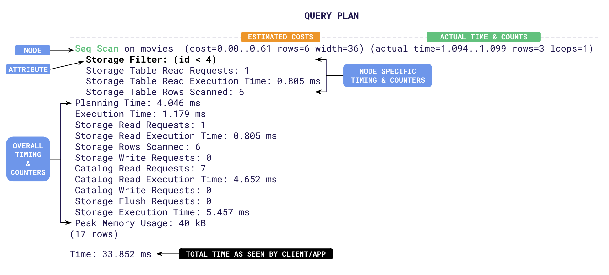
The output is effectively the plan tree followed by a summary of timing and counters. Each line represents a step (a.k.a node) involved in processing the query. The top line shows the overall plan and its estimated cost. Subsequent indented lines detail sub-steps involved in the execution. The structure of this output can be complex but contains valuable information to understand how YugabyteDB processes a query. Let's break down the typical structure of the EXPLAIN ANALYZE output:
- **Node Information**: Each line of the output represents a node in the query execution plan. The type of node and the operation it performs are typically indicated at the beginning of the line, for example, _Seq Scan_, _Index Scan_, _Nested Loop_, _Hash Join_, and so on.
- **Cost and Row Estimates**:
- _cost_ attribute is the estimated cost of the node's operation according to YugabyteDB's query planner. This cost is based on factors like I/O operations, CPU usage, and memory requirements.
- _rows_ attribute is the estimated number of rows that will be processed or returned by the node.
- **Actual Execution Statistics**:
- _time_: The actual time taken to execute an operation represented by the node during query execution. This is represented in two parts as _T1..T2_ with T1 being the time taken to return the first row, and T2 the time taken to return the last row.
- _rows_: The actual number of rows processed or returned by the node during execution.
- **Other Attributes**: Some nodes may have additional attributes depending on the operation they perform. For example:
- _Filter_: Indicates a filtering operation.
- _Join Type_: Specifies the type of join being performed (for example, Nested Loop, Hash Join, Merge Join).
- _Index Name_: If applicable, the name of the index being used.
- _Sort Key_: The key used for sorting if a sort operation is involved.
- _Sort Method_: The sorting algorithm used (for example, _quicksort_, _mergesort_, and so on.)
- **Timings**: At the end of the plan tree, YugabyteDB will add multiple time taken metrics when the [DIST](../../../../api/ysql/the-sql-language/statements/perf_explain/#dist) option is specified. These are aggregate times across all plan nodes. Some of them are,
- _Planning Time_: The time taken in milliseconds for the [query planner](../../../../architecture/query-layer/#planner) to design the plan tree. Usually this value is higher the first time a query is executed. During subsequent runs, this time will be low as the plans are cached and re-used.
- _Execution Time_: The total time taken in milliseconds for the query to execute. This includes all table/index read/write times.
- _Storage Read Execution Time_: The total time spent by the YSQL query layer waiting to receive data from the DocDB storage layer. This is measured as the sum of wait times for individual RPCs to read tables and indexes. The YSQL query layer often pipelines requests to read data from the storage layer. That is, the query layer may choose to perform other processing while a request to fetch data from the storage layer is in progress. Only when the query layer has completed all such processing does it wait for the response from the storage layer. Thus the wait time spent by the query layer (_Storage Read Execution Time_) is often lower than the sum of the times for round-trips to read tables and indexes.
- _Storage Write Execution Time_: The sum of all round-trip times taken to flush the write requests to tables and indexes.
- _Catalog Read Execution Time_: Time taken to read from the system catalog (typically during planning).
- _Storage Execution Time_ : Sum of _Storage Read_, _Storage Write_ and _Catalog Read_ execution times.
- _Time_: The total time taken by the request from the view point of the client as reported by ysqlsh. This includes _Planning_ and _Execution_ times along with the client to server latency.
- **Distributed Storage Counters**: YugabyteDB adds specific counters related to the distributed execution of the query to the summary when the [DIST](../../../../api/ysql/the-sql-language/statements/perf_explain/#dist) option is specified. Some of them are:
- _Storage Table Read Requests_: Number of RPC round-trips made to the local [YB-TServer](../../../../architecture/yb-tserver) for main table scans.
- _Storage Table Rows Scanned_: The total number of rows visited in tables to identify the final result set.
- _Storage Table Writes_ : Number of requests issued to the local [YB-TServer](../../../../architecture/yb-tserver) to perform inserts/deletes/updates on a non-indexed table.
- _Storage Index Rows Scanned_: The total number of rows visited in indexes to identify the final result set.
- _Storage Index Writes_ : Number of requests issued to the local [YB-TServer](../../../../architecture/yb-tserver) to perform inserts/deletes/updates on an index.
- _Storage Read Requests_: The sum of number of _table reads_ and _index reads_ across all plan nodes.
- _Storage Rows Scanned_: Sum of _Storage Table/Index_ row counters.
- _Storage Write Requests_: Sum of all _Storage Table Writes_ and _Storage Index Writes_.
- _Catalog Read Requests_: Number of requests to read catalog information from [YB-Master](../../../../architecture/yb-master).
- _Catalog Write Requests_: Number of requests to write catalog information to [YB-Master](../../../../architecture/yb-master).
- _Storage Flush Requests_: Number of times buffered writes have been flushed to the local [YB-TServer](../../../../architecture/yb-tserver).
## Using explain
The following examples show how to improve query performance using output of the `EXPLAIN ANALYZE`. First, set up a local cluster for testing out the examples.
{{}}
### Set up tables
1. Create a key value table as follows:
```sql
CREATE TABLE kvstore (
key VARCHAR,
value VARCHAR,
PRIMARY KEY(key)
);
```
1. Add 10,000 key-values into the tables as follows:
```sql
SELECT setseed(0.5); -- to help generate the same random values
INSERT INTO kvstore(key, value)
SELECT substr(md5(random()::text), 1, 7), substr(md5(random()::text), 1, 10)
FROM generate_series(1,10000);
```
1. Run the [ANALYZE](../../../../api/ysql/the-sql-language/statements/cmd_analyze/) command on the database to gather statistics for the query planner to use.
```sql
ANALYZE kvstore;
```
## Speed up lookups
Use `EXPLAIN` on a basic query to fetch a value from the `kvstore` table.
{{}}
For brevity, all the output for the following examples excludes metrics/counters with value zero. `COSTS OFF` option has also been added to show just the estimated costs.
{{}}
```sql
EXPLAIN (ANALYZE, DIST, COSTS OFF) select value from kvstore where key='cafe32c';
```
You should see an output similar to the following:
```yaml{linenos=inline, .nocopy}
QUERY PLAN
-------------------------------------------------------------------------------------
Index Scan using kvstore_pkey on kvstore (actual time=1.087..1.090 rows=1 loops=1)
Index Cond: ((key)::text = 'cafe32c'::text)
Storage Table Read Requests: 1
Storage Table Read Execution Time: 0.971 ms
Storage Table Rows Scanned: 1
Planning Time: 0.063 ms
Execution Time: 1.150 ms
Storage Read Requests: 1
Storage Read Execution Time: 0.971 ms
Storage Rows Scanned: 1
Storage Execution Time: 0.971 ms
```
From line 3, you can see that an index scan was done on the table (via `Index Scan`) using the primary key `kvstore_pkey` to retrieve one row (via `rows=1`). The `Storage Rows Scanned: 1` indicates that as only one row was looked up, this was an optimal execution.
Fetch the key for a given value:
```sql
EXPLAIN (ANALYZE, DIST, COSTS OFF) select * from kvstore where value='85d083991d';
```
You should see an output similar to the following:
```yaml{linenos=inline, .nocopy}
QUERY PLAN
-------------------------------------------------------------------
Seq Scan on kvstore (actual time=3.719..3.722 rows=1 loops=1)
Storage Filter: ((value)::text = '85d083991d'::text)
Storage Table Read Requests: 1
Storage Table Read Execution Time: 3.623 ms
Storage Table Rows Scanned: 10000
Planning Time: 1.176 ms
Execution Time: 3.771 ms
Storage Read Requests: 1
Storage Read Execution Time: 3.623 ms
Storage Rows Scanned: 10000
Catalog Read Requests: 1
Catalog Read Execution Time: 0.963 ms
Storage Execution Time: 4.586 ms
```
Immediately from line 3, you can see that this was a sequential scan (via `Seq Scan`). The `actual rows=1` attribute indicates that only one row was returned, but `Storage Rows Scanned: 10000` on line 12 indicates that all the 10,000 rows in the table were looked up to find one row. So, the execution time `3.771 ms` was higher than the previous query. You can use this information to convert the sequential scan into an index scan by creating an index as follows:
```sql
CREATE INDEX idx_value_1 ON kvstore(value);
```
If you run the same fetch by value query, you should see an output similar to the following:
```yaml{linenos=inline, .nocopy}
# EXPLAIN (ANALYZE, DIST, COSTS OFF) select * from kvstore where value='85d083991d';
QUERY PLAN
-----------------------------------------------------------------------------------
Index Scan using idx_value_1 on kvstore (actual time=1.884..1.888 rows=1 loops=1)
Index Cond: ((value)::text = '85d083991d'::text)
Storage Table Read Requests: 1
Storage Table Read Execution Time: 0.861 ms
Storage Table Rows Scanned: 1
Storage Index Read Requests: 1
Storage Index Read Execution Time: 0.867 ms
Storage Index Rows Scanned: 1
Planning Time: 0.063 ms
Execution Time: 1.934 ms
Storage Read Requests: 2
Storage Read Execution Time: 1.729 ms
Storage Rows Scanned: 2
Storage Execution Time: 1.729 ms
Peak Memory Usage: 24 kB
```
In this run, Index scan was used and the execution time has been lowered (`1.934 ms` - 40% improvement). Only one row was returned (via `rows=1`), but two rows were scanned (`Storage Rows Scanned: 2`) as one row was looked up from the index (via `Storage Index Rows Scanned: 1`) and one row was looked up from the table (via `Storage Table Rows Scanned: 1`). This is because, the executor looked up the row for the matching value: `85d083991d` from the index but had to go to the main table to fetch the key, as we have specified `SELECT *` in our query. Only the values are present in the index and not the keys.
You can avoid this by including the `key` column in the index as follows:
```sql
CREATE INDEX idx_value_2 ON kvstore(value) INCLUDE(key);
```
If you run the same fetch by value query, you should see an output similar to the following:
```yaml{linenos=inline, .nocopy}
# EXPLAIN (ANALYZE, DIST, COSTS OFF) select * from kvstore where value='85d083991d';
QUERY PLAN
----------------------------------------------------------------------------------------
Index Only Scan using idx_value_2 on kvstore (actual time=1.069..1.072 rows=1 loops=1)
Index Cond: (value = '85d083991d'::text)
Storage Index Read Requests: 1
Storage Index Read Execution Time: 0.965 ms
Storage Index Rows Scanned: 1
Planning Time: 0.074 ms
Execution Time: 1.117 ms
Storage Read Requests: 1
Storage Read Execution Time: 0.965 ms
Storage Rows Scanned: 1
Storage Execution Time: 0.965 ms
```
Notice that the operation has become an `Index Only Scan` instead of the `Index Scan` as before. Only one row has been scanned (via `Storage Rows Scanned: 1`) as only the index row was scanned (via `Storage Index Rows Scanned: 1`). The execution time has now been lowered to `1.117 ms`, a 40% improvement over previous execution.
## Optimizing for ordering
Fetch all the values starting with a prefix, say `ca`.
```sql
EXPLAIN (ANALYZE, DIST, COSTS OFF) SELECT * FROM kvstore WHERE value LIKE 'ca%' ORDER BY VALUE;
```
You should see an output similar to the following:
```yaml{linenos=inline, .nocopy}
QUERY PLAN
-----------------------------------------------------------------------------
Sort (actual time=4.007..4.032 rows=41 loops=1)
Sort Key: value
Sort Method: quicksort Memory: 28kB
-> Seq Scan on kvstore (actual time=3.924..3.957 rows=41 loops=1)
Storage Filter: ((value)::text ~~ 'ca%'::text)
Storage Table Read Requests: 1
Storage Table Read Execution Time: 3.846 ms
Storage Table Rows Scanned: 10000
Planning Time: 1.119 ms
Execution Time: 4.101 ms
Storage Read Requests: 1
Storage Read Execution Time: 3.846 ms
Storage Rows Scanned: 10000
Catalog Read Requests: 1
Catalog Read Execution Time: 0.877 ms
Storage Execution Time: 4.723 ms
```
Only 41 rows were returned (`rows=41`) but a sequential scan (`Seq Scan on kvstore`) was performed on all the rows (`Storage Rows Scanned: 10000`). Also, the data had to be sorted (via `Sort Method: quicksort`) on value (via `Sort Key: value`). You can improve this execution by modifying the above created index into a range index, so that you can avoid the sorting operation, and reduce the number of rows scanned.
```sql
CREATE INDEX idx_value_3 ON kvstore(value ASC) INCLUDE(key);
```
If you run the same query, you should see the following output:
```yaml{linenos=inline, .nocopy}
# EXPLAIN (ANALYZE, DIST, COSTS OFF) SELECT * FROM kvstore WHERE value LIKE 'ca%' ORDER BY VALUE;
QUERY PLAN
-----------------------------------------------------------------------------------------
Index Only Scan using idx_value_3 on kvstore (actual time=0.884..0.935 rows=41 loops=1)
Index Cond: ((value >= 'ca'::text) AND (value < 'cb'::text))
Storage Filter: ((value)::text ~~ 'ca%'::text)
Storage Index Read Requests: 1
Storage Index Read Execution Time: 0.792 ms
Storage Index Rows Scanned: 41
Planning Time: 4.290 ms
Execution Time: 1.008 ms
Storage Read Requests: 1
Storage Read Execution Time: 0.792 ms
Storage Rows Scanned: 41
Catalog Read Execution Time: 3.824 ms
Storage Execution Time: 4.616 ms
```
Now, only 41 rows were scanned (via `Storage Rows Scanned: 41`) to retrieve 41 rows (via `rows=41`) and there was no sorting involved as the data is stored sorted in the range index in `ASC` order. Even though YugabyteDB has optimizations for reverse scans, if most of your queries are going to retrieve the data in `DESC` order, then it would be better to define the ordering as `DESC` when creating a range sharded table/index.
## Learn more
- Refer to [Get query statistics using pg_stat_statements](../pg-stat-statements/) to track planning and execution of all the SQL statements.
- Refer to [View live queries with pg_stat_activity](../../../../explore/observability/pg-stat-activity/) to analyze live queries.
- Refer to [View COPY progress with pg_stat_progress_copy](../../../../explore/observability/pg-stat-progress-copy/) to track the COPY operation status.
- Refer to [Optimize YSQL queries using pg_hint_plan](../pg-hint-plan/) to show the query execution plan generated by YSQL.